Only use for SAP HANA based applications, not legacy SAP applications which make use of MSSQL, Oracle etc.
Multi-node SAP scale-out is not supported (used for larger SAP BW instances)
This sizing process does not vary for scale-up between AHV & VMware implementations
No spinning disks are used within a Nutanix cluster being used for SAP HANA
Any questions, support, or areas not covered – please use the SAP Slack channel
Supported Platforms:
Only Dell, HPE, Fujitsu and Lenovo are supported for SAP HANA, not NX.
If another OEM is selected, SAP HANA will not be shown as an available workload
Defaults
RF2 is used (RF3 is under testing, so not selectable in Sizer)
Compression is disabled, and not typically of value for SAP HANA
Higher default CVM resource is reserved
HANA Inputs
NVMe can be added for higher IO loads, such as a high usage SAP S4/HANA
Cost/Performance largely drives cpu choice. Ideally an implementation’s potential compute load in SAPS would be known. Please reach out for support in estimating and reviewing such information.
Environments
There would typically be two environments within a Nutanix cluster where production and non-production are mixed. Production rules should be applied both to all production instances, and any other instances that should be treated as production. This might apply to a QAS/Test environment and will typically apply to any DR cluster.
Production:
For most SAP applications (e.g., production S4) there is an SAP HANA database, and one or more application server instances. Some uses of SAP HANA do not use an application server, in which case just use a small one in the sizing exercise.
In addition to the Application Server instances, and the SAP HANA database, a small VM called the ASCS is often called for. This ASCS would be around 2c/24GB RAM/100GB disk.
Generally, production has two or more application server instances. Typically, 2 – 6 cores, with around 24GB/core. Multiple instances for larger loads. Small storage space requirement for os & application image.
For a downtime requirement of less than 20 minutes, a pair of SAP HANA instances should be sized.
There is no over commit of cpu or memory
Servers must have all memory channels filled and balanced, so 6 or 12 DIMMs per cpu. – Sizer auto recommendation enforces this consideration
L suffix cpus are required for largest memory instances
Available storage for SAP HANA should be around 2.5x to 3x memory (3x is used in Sizer)
Production rules – SAP HANA instances are on whole dedicated cpus and so cannot be allocated to the CVM cpu
HANA System Relication(HSR) – is exactly a copy of the HANA VM. In Sizer, add another HANA VM if implementing the HSR.
Non Production:
QAS/Test landscape tends to match nonPRD for size of instance
If an operating system HA cluster is used in production, there is typically at least one such cluster outside of production also – used as a testbed.
Each SAP solution would normally have two or three non-production landscapes
Solution Manager (SolMan) is often overlooked, and not asked for. It is a required instance in the overall deployment and would be sized in PRD with one SAP HANA instance and an application server instance. Another such pair for QAS/test. No HA clustering would be required.
DEV, SBX etc. are usually subsets in memory size.
Feb 8, 2021
First release of SAP HANA in the sizer:
Tendency to move to four socket servers when two socket my suffice.
You may observer this , however, this would largely be because of the DIMMs cost considerations between a 24x64GB and 48x32GB
This is the most common workload along with VDI. This can be used for any web app which needs to be sized. Each workload or the application which is to be migrated to the Nutanix software stack is a VM with its own CPU/RAM/Capacity requirements. To simplify for the users, Sizer has set profiles (small,medium,large ) for the VMs but customizable as per the actual application needs.
What are profiles in Server Virtualization in Sizer?
Profiles are fixed templates with pre assigned resources in terms of vCPUs, RAM, SSD, HDD to each profile. Broadly, small, medium,large profiles will have different allocation of these resources.
The idea is to facilitate users with the details of a workload (that is a VM) so they cna quickly fill in number of VMs and Sizer will do the necessary sizing.
Small VM profile template:
Medium VM profile template:
Large VM profile template:
What if my VMs are different? Have differen values?
While these templates and their values are general guidelines, these are customisable.
Clicking on the Customize, opens a pop-up for user entered values:
The Nutanix platform leverages a replication factor (RF) for data protection and availability. This method provides the highest degree of availability because it does not require reading from more than one storage location or data re-computation on failure. However, this does come at the cost of storage resources as full copies are required.
To provide a balance between availability while reducing the amount of storage required, DSF provides the ability to encode data using erasure codes (EC). Similar to the concept of RAID (levels 4, 5, 6, etc.) where parity is calculated, EC encodes a strip of data blocks on different nodes and calculates parity. In the event of a host and/or disk failure, the parity can be leveraged to calculate any missing data blocks (decoding).
The number of data and parity blocks in a strip is configurable based upon the desired failures to tolerate. The configuration is commonly referred to as the number of <data blocks>/<number of parity blocks>.
How is ECX savings calculated in Sizer ?
Sizer follows the Nutanix Bible and its guidelines for ECX savings.
Below table shows the ECX overhead vs RF2/RF3 for different nodes:
The expected overhead can be calculated as <# parity blocks> / <# data blocks>. For example, a 4/1 strip has a 25% overhead or 1.25X compared to the 2X of RF2. A 4/2 strip has a 50% overhead or 1.5X compared to the 3X of RF3.
How does Sizer calculate ECX savings from the above:
Lets take an example where the cold data for workload is 100TiB.
Also, we will use RF2 as the settings chosen for workload.
So depending on the size of the workload, if the total node recommended came to (lets say 4 nodes), as per the above table: data/parity is 2/1. So 1.5x overhead for ECX as against 2 for RF2 , thus 50% savings.
For conservative approach and to be on safe side, we only consider ECX for 90 % of the cold data.
Sizer focuses on both the sizing and the license aspects of using Era to manage your databases that are defined in Sizer. So for a long time you could size either Oracle or SQL databases a customer may want to run on a Nutanix cluster. With Era you can manage those databases but also set up data protection policy and manage clones. Sizer then does the following in regards to Era that is turned on for either Oracle or SQL workloads
Determine the licensing required for the Oracle or SQL VMs defined in Sizer. Era is VCPU based and so number of VCPUs under management
Determine all the sizing requirements for the data protection policy defined in the workload including time machine requirements
Determine the cloning requirements (if enabled) for either database only (just storage) clones or the database plus VM clones (entire database VM clone)
Determine the sizing requirements for Era VM itself
Era License/Sizing
Let’s say you just want to buy Era for the Oracle workloads but not snapshots or clones. In next sections we will deal with database protection policy and cloning. So here we just want to add the Era licenses
Here is the setting in the Oracle workload. We are saying here we want Era for all 10 Oracle VMs and each VM has 8 VCPUs. Coincidentally it is VCPU:pCore of 1:1 and so 8 cores. Era licensing though is VCPUs
Here is the budgetary quote and indeed shows 80 VCPUs must be licensed.
Here is the Era sizing. We do add the VM to run Era which is lightweight
Era Data Protection including Time Machine
To invoke data protection Era must be enabled and the licensing is scoped as described above.
Sizer will now let you define the data protection policy you would define in Era and figure out the sizing requirements.
Daily Database Change rate can either be in % or in GiB but is the amount of change per day for the databases defined in the workload (the database VMs defined in the workload)
Daily log size is either % or GiB. This is used by Time Machine to allow for continuous recovery for the time frame specified. All the transactions are logged and Time Machine can allow for rollback to a given point in time
Continuous Snapshots is in days
Daily, Weekly, Monthly, and Quarterly are number of snapshots kept for snapshots done in those time frames
Here are the sizing results.
Era VM – the logs are kept by the Era VM in SSD. This is for Time Machine to do continuous recovery
The other snapshots are put in cold storage and like anything stored in a cluster has its RF overhead (here it is set to RF2).
Should note the quarterly snapshots add a lot of storage
Era Database Only Clones
You can define cloning policy in Era and thus in Sizer so it can calculate the sizing requirement
Define number of clones for all the database VMs in the workload. Here we had 10 VMs and so 2 clones per VM
Clone daily change rate – this would be the % or GiB change each day by typically developers that are using those clones.
Refresh rate. At some point (in days) organizations typically refresh the clones with new data and so represents maximum time the clones are kept
Here is the sizing. Note the impact is Era DB only clone is added in the workload summary and the just the capacity is added. All the calculations form the Era data protection policy is not impacted
Era DB plus VM clones
Here we add in clones of the VMs and so the storage and VMs themselves
Define number of clones for all the database VMs in the workload. Here we had 10 VMs and so 2 clones per VM
Clone daily change rate – this would be the % or GiB change each day by typically developers that are using those clones.
Refresh rate. At some point (in days) organizations typically refresh the clones with new data and so represents maximum time the clones are kept
VCPU per VM. In the workload we defined a database VM needed 8 VCPUs. Well if this clone is test/dev it could be less
VCPU:pCore ratio. In workload it is 1:1 but for test/dev 2:1 is more common
RAM per VM is needed
Here is the sizing. Note the impact is Era DB Plus VM Clone is added in the workload summary. Where for the Era DB Only Clone it is just added capacity, the Era DB Plus VM Clone adds VMs.
20 VMs were added as we have 10 VMs in the workload and we asked for 2 clones per source database
80 cores are needed as those 20 VMs need 8 VCPUs but we specified 2:1 VCPU:pCore ratio. Thus 160 more VCPUs but just 80 cores. Do note those VCPU’s are added into the Era licensing as Era is managing those VCPUs.
We need 2.5 TiB of RAM as we have 20 VMs and each needs 128 GiB
Capacity is same as what we had for the DB only clone as same settings
All the calculations form the Era data protection policy is not impacted
Now Sizer provides an option to select the type of processor the workload (existing or proposed) is running on. This gets factored in while sizing for the workload adding precision to the sizing and overall recommendation.
To give an example of how it helps.. an existing worklaod (say Server Virt, 100 of them) running on a weak processor (say a Haswell 2699v3, specint-38.58) would require less cores in sizing than the same 100 VMs running on a high performing CPU( like Skylake 8156 specInt -68.85).
Previously, the processor for existing workload was not taken into account, though Sizer always used a baseline processor[E5 2680v2] . So irrespective of whether the current worklaod is running on a slowest processor or the fastsest one, sizings used to remain the same.
With this new addition, there is a lot more precision added to sizing as we account for the incremental changes due to different type of processors.
How do we handle the processor input during sizing?
Here is an example: input processor Broadwell E5 2690v4[46.43 specInt]
Lets say sizing comes to 32 cores
This sizing is at the baseline [E5 2680v2, 42.31 specInt] – Sizer defualt used until now
This has to be adjusted against the input processor E5 2690v4
32*[46.43/42.31] = 35.11
The way to read this:
If your existing processor was E5 2680v2(42.31), then the workload would require 32 cores
If your existing processor(E5 2690v4) is stronger than the above baseline (specInt wise), you would need more cores
Where do we select the processor input for the workload?
In the page where we give the workload name and select the type of workload, there is a dropdown to select the processor the workload is running on.
Currently, we support only one processor type per workload , however, there are chances that sometimes a workload can be running on mixed CPUs. In that case, it is advisable to go with the processor with better performance among the two.
Please note: This feature only deals with sizing based on the selected processor. It does not reflect or has any influence on the type of processor chosen for the recommended hardware. The HW recommendation continues to be driven based on the optimal HW solution based on the resources required (cores/flash/capacity)
In the past object storage solutions were only concerned with capacity; performance was barely a consideration. However, modern workloads such as AI/ML and data analytics leverage S3 compatible storage, and these very often have significant performance demands. Nutanix Objects has been internally benchmarked with both hybrid and all flash systems (see https://portal.nutanix.com/page/documents/solutions/details?targetId=TN-2098-Nutanix-Objects-Performance-INTERNAL-ONLY:TN-2098-Nutanix-Objects-Performance-INTERNAL-ONLY) and as a result we have a good understanding into Objects’ performance capabilities with a variety of workload profiles. Extrapolations can reliably be taken from these results to model performance scaling, since Objects I/O performance scales linearly. Importantly, the empirical data gleaned from the benchmark testing is leveraged by Sizer to determine the minimum number of Objects workers – and therefore nodes (Objects enforces 1 worker per node per object store for HA reasons) – needed to deliver a certain level of performance.
It should also be noted that there are factors outside the object store, such as network speed and number of client connections, that play a significant role in achieving the best possible performance from Nutanix Objects. Regarding the number of client connections, it should be noted that each node/worker needs 60-75 concurrent client connections driving I/O for maximum performance potential to be realized.
More commonly, node count will be driven by capacity requirements. Even in these cases however, the minimum Objects worker count needed for the required performance should still be noted, especially in mixed deployments (discussed further below).
Configurations
While there is no difference in NUS licensing between dedicated deployments (the AOS cluster is dedicated to NUS) and mixed deployments (NUS resides on the same cluster as application VMs), sizing considerations in each scenario vary to a degree. These are discussed below.
Worker count and HDD spindle count (or SSD count if All Flash)
In scenarios where a certain level of performance must be met, Sizer will look at the number of workers needed and the number of HDDs (or SSDs in the case of all flash) needed to deliver the throughput entered*. A high performance worker on an all flash node can, in most scenarios, deliver substantially more throughput than a standard worker on a hybrid node.
Disk-wise, in RF2 configs Sizer assumes a single SATA HDD can deliver reads:100MB/s and writes:50MB/s. Sizer assumes a single SSD can deliver reads:500MB/s and writes:250MB/s. So for example, a hybrid node with 10*HDDs can deliver 1GB/s for a workload consisting entirely of reads, or 500MB/s for a workload consisting entirely of writes. If RF3 or FT1n/2d is selected the write throughput figure is increased by 50% to account for the additional disk write IO. Note that FT1n/2d is strongly recommended for storage dense configs.
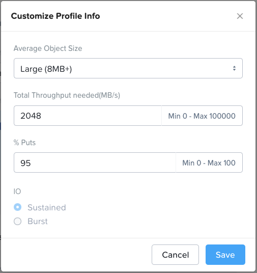
*For performance sensitive sizings please do not just accept the default values in the performance profile section (“Profile Info” box in the top right of the Workload page). The default values are purely arbitrary. You must determine the actual average object size, R/W (get/put) split and throughput that the customer needs to achieve and enter that customer-specific data into the Profile Info section.
For an Objects dedicated configuration (hybrid)
Objects is supported on all models and platforms that can run AOS (NCI). However, if you’re sizing for a dedicated hybrid Objects cluster with 100TiB or above, we recommend the HPE DX4120-G11, NX-8155-G9 or equivalent for the best performance. Such models are ideal due to their high HDD spindle count (as discussed in the previous section), though any model will work as long as it matches the minimum configurations listed below.
CPU: dual-socket 12-core CPU (minimum) for hybrid configs with 4 or more HDDs
Dual-socket 10-core CPU is acceptable for hybrid configs in use cases that do not require fast performance
Memory: 128GB per node (minimum)
Disk:
Avoid hybrid configurations that have only 2 HDDs per node.
For hybrid configurations that need to deliver good throughput, systems with 10+ HDDs are highly recommended. On an NX8155 for example go for 2*SSD + 10*HDD rather than 4*SSD + 8*HDD. This is further explained in the below section Why 10+ HDDs in a dedicated hybrid config?
If a system with 10 or more HDDs is not available, configure the system with the highest number of HDDs possible.
Erasure Coding: inline enabled (set by default during deployment)
Note inline EC has a 10-15% impact on write performance (accounted for if you choose “inline EC” in Sizer)
FT choice: choosing between RF3, FT1N/2D and RF3 has an impact on the system’s deliverable write throughput (see previous section “Worker count and HDD spindle count (or SSD count if All Flash)”)
Network: dual 25GbE generally recommended (but check calculation in “Network” section)
NOTE: In Sizer to force a hybrid cluster output make sure “Hybrid” is selected under “Worker Node”. Sizer does not automatically choose between hybrid or all-flash for you.
Licensing: NUS Starter covers any Objects deployment on a hybrid system (whether shared or dedicated).
Why 10+ HDDs in a dedicated hybrid config?
In the majority of today’s use cases objects tend to be large (>1.5MiB), meaning they manifest as sequential I/O on the Nutanix cluster. In response to this, Objects architecture is tuned to take full advantage of the HDD tier. If there are HDDs in a node, Objects will automatically write sequential data directly to them, while leveraging the SSDs purely for metadata (if there are any objects under 1.5MB these will land in the SSD tier).
There are 3 reasons for this;
Solid sequential I/O performance can be achieved with HDDs, assuming there are enough of them
Objects deployments can be up to petabytes in size. At that sort of scale, cache or SSD hits are unlikely, so using SSDs in hopes of achieving accelerated performance through caching would provide little return on the additional costs. To keep the solution cost-effective, Objects minimizes SSD requirements by using SSDs for metadata, and only using for data if required.
Since we recommend a dual-socket 12-core CPU configuration, fewer SSDs also helps to avoid system work that would otherwise be incurred by having to frequently move data between tiers – the result is less stress on the reduced CPU count.
If, however, the workload is made up of mostly small objects, all-flash systems are significantly better at catering for the resulting random I/O, particularly if the workload is performance intensive.
For an Objects dedicated configuration (all-flash)
If all-flash is the preference, any system with 3 or more SSD/NVMe devices is generally fine, although the calculation described earlier must be performed based on actual throughput requirements (Sizer does this). If the all-flash nodes must also be storage dense we recommend the NX-8150-G9. From a compute standpoint, all-flash Objects clusters should have a minimum of:
CPU: dual-socket 20-core CPU (minimum) for all-flash configs – importantly, this allows the “Performance Config” to be selected at deployment
Memory: 128GB per node (minimum)
Disk: For all flash configurations, systems with 3 SSDs/NVMes (or more) are recommended.
Erasure Coding: inline enabled (set by default during deployment)
Note inline EC has a 10-15% impact on write performance (accounted for if you choose “inline EC” in Sizer)
FT choice: choosing between RF3, FT1N/2D and RF3 has an impact on the system’s deliverable write throughput (see previous section “Worker count and HDD spindle count (or SSD count if All Flash)”)
Network: quad 25GbE, dual 40GbE or higher generally recommended, and for very high performance requirements dual 100GbE will be needed (check calculation in “Network” section)
NOTE: In Sizer to force an all-flash cluster output make sure “All Flash” is selected under “Worker Node”. Sizer does not automatically choose between hybrid or all-flash for you.
Licensing: NUS Pro covers any Objects deployment on an all flash system (whether shared or dedicated).
For a mixed configuration (Objects coexisting with User VMs)
Objects is supported on any model and any platform as long as it matches the minimum configurations listed below.
CPU: at least 12 vCPUs are available per node
All node types with dual-socket CPUs are supported and preferred, though single CPUs with at least 24 cores are also supported
Memory: at least 36GB available to Objects per node
Disk: avoid hybrid configurations with only 2 HDDs per node and bear in mind that more HDD spindles means better performance.
Erasure Coding: Inline enabled (set by default during deployment)
Note inline EC has a 10-15% impact on write performance (accounted for if you choose “inline EC” in Sizer)
FT choice: choosing between RF3, FT1N/2D and RF3 has an impact on the system’s deliverable write throughput (see previous section “Worker count and HDD spindle count (or SSD count if All Flash)”)
Network: dual 25GbE recommended (but check calculation in “Network” section)
Both the NUS Starter and Pro licenses allow one User VM (UVM) per node. If taking advantage of this, ensure that there are enough CPU cores and memory on each node to cater for both an Objects worker and the UVM – and potentially also a Prism Central (PC) VM, unless PC will be located on a different cluster. It’s important to understand that Nutanix Objects cannot be deployed without there being a Prism Central present somewhere in the environment.
Network
This section provides information on working out the network bandwidth (NIC speed and quantity) needed per node, given the customer’s throughput requirement and the number of load balancers in the deployment. Conversely, it can be used to work out how many load balancers are needed, particularly if the customer is limited to a particular speed of network. At the end of this section is a link to a spreadsheet that helps you perform these calculations.
Note that Sizer does not perform these calculations. Sizer will statically configure all-flash Object nodes with 4 x 25GbE ports (two dual port cards). However, that might not be enough so it’s important that you do the performance calculations below and, if necessary, manually increase the NIC speed and/or quantity in Sizer as needed.
1. Firstly it’s important to be aware that for each put (write) request received by Objects there is 4x network amplification. The write path is as follows:
Client > Load Balancer (1) > Worker (2) > CVM (3) > RF write to another CVM (4)
If RF3 or 1N2D is selected this increases to 5x network amplification
For each get (read) request received there is 3x amplification. The read path is as follows:
CVM > Worker (1) > Load Balancer (2) > Client (3)
If EC is selected (EC is default if there are enough nodes) read amplification could, for many gets, increase to 4x if parts of the EC strip need to be read from other CVMs.
So the total network bandwidth needed for the object store is determined by the customer’s requested throughput multiplied by these factors in the correct proportions (R/W). The resulting overall bandwidth requirement is then spread across the load balancers – a relatively even distribution is assumed.
2. Take whatever % of the customer’s throughput is write IO (puts) – this is typically expressed in MB/s or GB/s – and multiply by 4 (or 5 – see above) to account for the write amplification. Next, take whatever % of the customer’s throughput is read IO (gets) and multiply that by 3 (or 4 – see above) to account for the read amplification. Combine the results and you have the overall throughput requirement to/from the cluster.
Total bandwidth to/from object store = 4 GB/s + 12 GB/s = 16 GB/s
3. Divide the overall throughput figure by the number of load balancers you plan to deploy. The result is the amount of network bandwidth needed per physical node.
Example:
4 Load Balancers
16 GB/s / 4 = 4 GB/s per node
4. Map this figure to the real world limits of NICs of varying speeds. These are listed below for your convenience. Note that when 2 links are aggregated using LACP you do not get twice the bandwidth of a single link due to overheads. With 2 links in LACP you can assume ~20% bandwidth loss, with 4 you can assume ~40% loss. Further to that, and before LACP overhead is accounted for, a NIC’s advertised bandwidth is never fully achievable due to general networking overheads (protocol and other real world factors).
# links in LACP
1 (no aggregation)
2
4
Achievable GB/s
1.1
1.8
2.7
Usable bandwidth with 10GbE
# links in LACP
1 (no aggregation)
2
4
Achievable GB/s
2.8
4.4
6.6
Usable bandwidth with 25GbE
# links in LACP
1 (no aggregation)
2
4
Achievable GB/s
4.4
7.0
10.4
Usable bandwidth with 40GbE
# links in LACP
1 (no aggregation)
2
4
Achievable GB/s
10.5
*12.5 (not 16.8)
*12.5 (not 25.2)
Usable bandwidth with 100GbE
*At the time of writing OVS, the virtual switch architecture used by AHV/KVM, has a limit of 100Gbps – this means the maximum network throughput a single node can handle is 12.5 GB/s (100/8). The configurations affected by this are 2x and 4x 100GbE links in LACP. There are future plans to lift this limit (roadmap item).
Example:
4 GB/s per node is needed.
Each node needs 2 x 25GbE NICs (in LACP), which can do 4.4GB/s
This spreadsheet may help with the network bandwidth and load balancer calculations.
Sizing Use Cases
Use Case: Backup
Below is a Backup workload in Objects Sizer. In this scenario Nutanix Objects is used as a target to store backups sent from backup clients (i.e. the backup app).
Note that Nutanix Objects should not be located on the same physical cluster as the source data (i.e. the data being backed up).
Considerations when sizing a backup workload
Initial capacity – estimated initial capacity that will be consumed by backups stored on Nutanix Objects.
Capacity growth – % growth of the backup data per time unit (e.g. years) over an overall specified length of time.
Be cautious and do not attempt to cater for too long a growth period, otherwise the amount of capacity required due to growth could dwarf the amount of storage required on day one. Specifying a (for example) 10-year growth period undermines our fundamental pay-as-you-grow value. Plus of course growth predictions may not be entirely accurate in any case. 3 years is a typical growth period to size for.
Do not enable Nutanix deduplication on any Objects workloads.
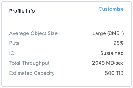
Profile Info:
All values can be customized as required.
Write (PUT) traffic usually dominates these environments as backups occur more regularly than restores (GETs). Furthermore, when restores do occur they are usually just reading a small subset of the backup.
That said, more and more customers are becoming increasingly concerned with how fast all their data could be restored in the event of a ransomware attack – so do check this with the customer
Backups usually result in sequential I/O so the requirement is expressed as MB/s throughput. Veeam is the one exception to this rule – discussed further below.
Backups usually consist of large objects (with the exception of Veeam – discussed further below)
“Sustained” only applies to small object (<1.5MB) puts. In a hybrid system, when the hot tier fills up the application I/O must wait while the data is drained from SSD/NVMe to HDD. This is why sustained small object put throughput is slower than burst small object put throughput.
Replication Factor
When using nodes with large disks (12TB+) to achieve high storage density it’s recommended you use RF3 or, better still, 1N/2D if there are 100 or more disks in a single fault domain. This provides a higher level of resilience against disk failure. Disk failure is more likely in this scenario for two reasons:
The more disk hardware you have the greater the risk of a disk failure
Disks take longer to rebuild because they contain more data, thus the window of vulnerability is extended (to days rather than hours)
The larger drive capacities also mean there is a greater chance of encountering a latent sector error (LSE) during rebuild
This drives a real need for protection against dual disk failure – true regardless of whether the disks are HDD or SSD/NVMe.
1N/2D coupled with wider EC strip sizes is preferred to RF3 due to it being more storage efficient
If you wish to stick with RF2, consider using multiple Objects clusters.
However each cluster will have its own N+1 overhead.
Special rules for Veeam
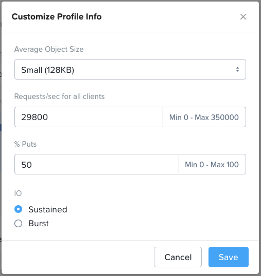
Veeam is different from other backup apps in that it does not write large objects. With Veeam the default object size is ~768KB, about a tenth (or less) of the size of objects generated by other backup apps. Therefore, for Veeam opportunities the specialized “Backup – Veeam” use case in Sizer should be selected. Note that small object performance requirements must be expressed in Sizer in requests/sec rather than MB/sec. Therefore some conversion may be required if the customer has provided a throughput number (the contrasting I/O gauges are discussed in the cloud-native apps section).
Because small objects will always hit the SSD/NVMe tier there is a danger the hot tier will fill up quickly causing Veeam to wait while the data is periodically drained to the HDDs. For this reason all-flash Objects is a better solution for Veeam, and is the default when the “Backup – Veeam” use case is selected.
If Commvault is the backup app, check whether the customer wishes to use both Commvault’s deduplication and WORM. If this is the case (and it often is), the storage requirement must be increased by 2.4x.
Archive is very similar to Backup and so the same advice applies. The profile values aren’t quite the same however, as you can see below. As with Backup though, these can be customized to the customer’s specific workload needs.
Use Case: Cloud-Native Apps
Cloud-native is a broad category covering a wide range of workload profiles. The correct I/O profile here depends on whether (and how) a containerized application will leverage Objects, or whether Objects is being deployed to support K8s management functions (or both). Object storage is commonly used in a K8s supportive role as an image registry, a log target and/or a backup repository. However, the cloud-native category can also include live application data, including anything from containerized big data/ analytics application data to vector database indexes and logs used in AI inference, all of which have intensive I/O requirements. For this reason, the default profile in Sizer (shown below) reflects a workload that’s performance sensitive in nature. Object size can also vary greatly in this category, but with many cloud-native workloads the object size will be much smaller than with traditional backup and archive workloads, so the profile defaults to a small object size. Smaller objects result in random I/O rather than sequential, and when this is the case all flash nodes are an infinitely better choice than hybrid. Note that this random I/O value is expressed in Sizer in requests/sec, rather than the MB/sec throughput metric that’s used to represent large object sequential I/O. These metrics are consistent with how random and sequential I/O respectively are normally gauged within industry.
When sizing Objects for a cloud-native app it’s important to try and find out from the customer what the I/O profile for the app is, then you can edit the I/O profile settings accordingly. This is especially important given the wide variance of cloud-native workloads types out there. In the absence of such information, all flash is the safe choice.
There is also a “Number of Objects (in millions)” field for all workload types. This is often relevant to cloud-native workloads (though not exclusively so), which can result in billions of objects needing to be stored and addressed. This value is used to determine how many Objects workers are needed to address the number of objects that will be stored. Thus, it could be that an Objects cluster sizing is constrained not by performance nor by capacity, but by metadata requirements.
What’s Missing from Sizer Today?
There are some sizing scenarios that are not currently covered by Objects Sizer. These are listed below, together with advice about what to do.
Sizing for intensive list activity
Szier cannot account currently for list activity. However, if you have been given a list requirement that you need to factor into your sizing, note that we have done benchmarking against list activity – the results can be viewed here.
Work with your local NUS SA to extrapolate these benchmarks to your customer’s requirement.
Objects sizes not currently represented in Sizer
Sizer currently only represents 128KB objects (small) and 8MB+ objects (large) – another object size is included (768KB) but it’s specifically for Veeam.
Small and large object workloads have very different performance profiles.
Objects from 8MB and above in size have a consistent performance profile, so select 8MB+ when you need to represent objects greater in size than 8MB, the output will be accurate. In Sizer, object size doesn’t matter above 8MB because you simply enter the overall throughput required (rather than requests/sec), together with the % puts (writes).
However, object sizes from 1KB right up to just under 8MB have logarithmically different performance profiles, meaning it is not easy to predict the performance of (for example) a 768KB object workload given what we know about 128KB performance and 8MB performance. Fortunately engineering has benchmark data for various object sizes other than 128KB and 8MB and this data can be used to identify a configuration that’s a closer fit to your customer’s specific object size. Work with your local NUS SA if you have this requirement. More object sizes will be added to Sizer in the future.
It’s again worth pointing out that objects >1.5MiB in size are classed by AOS as sequential I/O and will go straight to the HDD tier. Objects of 1.5MB or less, on the other hand, are classed as random I/O and will go straight to the SSD/NVMe tier. Knowing your customer’s object size in light of this fact is a significant factor (though not the only one) in helping you understand whether hybrid or all-flash is likely to be the better option.
Veeam and Commvault
These backup apps have additional considerations that can significantly affect the Objects cluster specification. You should not expect a straightforward ‘vanilla’ Backup sizing to be appropriate for these. Veeam is less of a challenge to size given that Sizer has a specialist category for Veeam workloads (“Backup – Veeam”). We are hoping to add a specialist Commvault category to Sizer in the future. In any case, please refer to the below documents when sizing Veeam or Commvault.
In case you are doing a manual sizing you want to make sure it meets N+1 resiliency.
This is easy to check and adjust if needed.
Go to manual sizing and decrement the node count.
Two things to keep in mind
The minimum number of nodes for Files is 4 as there is a FSVM on three nodes and 4th node is needed for N+1 (one node can be taken offline and still 3 nodes to run the 3 FSVMs). So 4 nodes are needed independent of capacity.
Second, like any Nutanix cluster you want to make sure you still are at N+1. Here is table that shows you max HDD utilization (Files is a HDD heavy workload) you want to assure N+1. For example, if you have 6 nodes and the HDD utilization is UNDER 75% you can be assured that you are at N+1. Here the N+0 target (utilization after lose a node) is 90%, meaning with a node offline the utilization is 90% or less.
Collector has a column “Workload Type” in the VMInfo tab where you can define the workload type for each VM. Currently, only two type of workload is supported – Server Virtualization or VDI. The defualt is set to Server Virtualization as this workload has been supported since beginning.
For VDI, you can go to each VM and change the Workload Type to VDI against each row.
Note: User has to explicitly go to each row and set the Workload Type as “VDI” .We will change it to dropdown to make it more intutive in future.
Defining the workload profiles
Each VM which is marked as VDI is bucketed into one of the 25 profiles based on the CPU(MHz) and RAM allocated to the VM.
CPU
Small <= (0-2000MHz)
Medium <= (2000-4000MHz)
Large <= (4000-8000MHz)
X-Large <= (8000 – 16000 MHz)
XX-Large <= (16000 – 32000 MHz)
RAM
Small = <1.024GB
Medium <2.048 GB
Large <8.2 GB
X-Large <16GB
XX-Large <32 GB
The 25 workload profiles based on the above.
VDI Small CPU Small RAM
VDISmall CPU Medium RAM
VDI Small CPU Large RAM
VDI Small CPU X-Large RAM
VDI Small CPU XX-Large RAM
VDI Medium CPU Small RAM
VDI Medium CPU Medium RAM
VDI Medium CPU Large RAM
VDI Medium CPU X-Large RAM
VDI Medium CPU XX-Large RAM
VDI Large CPU Small RAM
VDI Large CPU Medium RAM
VDI Large CPU Large RAM
VDI Large CPU X-Large RAM
VDI Large CPU XX-Large RAM
VDI X-Large CPU Small RAM
VDI X-Large CPU Medium RAM
VDI X-Large CPU Large RAM
VDI X-Large CPU X-Large RAM
VDI X-Large CPU XX-Large RAM
VDI XX-Large CPU Small RAM
VDI XX-Large CPU Medium RAM
VDI XX-Large CPU Large RAM
VDI XX-Large CPU X-Large RAM
VDI XX-Large CPU XX-Large RAM
Storage for each workload profile is calculated by adding the capacity for each VM in that profile (same as done for Server Virtualization)
Sizer asks for the VDI attributes upon Collector import:
Defualt values already selected.
The default values ( or user selected values ) captured here becomes the basis for initial VDI sizing.
Edit workload :
User can go to each VDI workload and make edits. However, this will overwrite the data collected from Collector (for ex: on capacity,ram etc) . The standard pre-defined templates ( defined in the normal VDI sizing) is applied once edited and parameters changed( like worker type, provision type, etc).
VM Performance data:
Collector also has performance data for the VMs collected over a 7 day period. The VM CPU utilization over past 7 days collected at 30 minute interval is collected and displayed. in the UI. While sizing, users can either go with allocated CPU or factor in the utilization rate to optimise on the overall CPU requirement for the VMs based on their historical usage. Basically, the utilization rate is a multiplier to the allocated CPU and a buffer is added to come up with net CPU. For more information on that, please refer to the Collector section.
Sizer relies on Login VSI profiles and tests. Here are descriptions about the profiles and applications run
Task Worker Workload
The Task Worker workload runs fewer applications than the other workloads (mainly Excel and Internet Explorer with some minimal Word activity, Outlook, Adobe, copy and zip actions) and starts/stops the applications less frequently. This results in lower CPU, memory and disk IO usage.
Below is the profile definition for a Task Worker:
Knowledge Worker Workload
The Knowledge Worker workload is designed for virtual machines with 2vCPUs. This workload contains the following applications and activities:
Outlook, browse messages.
Internet Explorer, browse different webpages and a YouTube style video (480p movie trailer) is opened three times in every loop.
Word, one instance to measure response time, one instance to review and edit a document.
Doro PDF Printer & Acrobat Reader, the Word document is printed and exported to PDF.
Excel, a very large randomized sheet is opened.
PowerPoint, a presentation is reviewed and edited.
FreeMind, a Java based Mind Mapping application.
Various copy and zip actions.
Below is the profile definition for a Knowledge Worker:
Power Worker Workload
The Power Worker workload is the most intensive of the standard workloads. The following activities are performed with this workload:
Begins by opening four instances of Internet Explorer which remain open throughout the workload.
Begins by opening two instances of Adobe Reader which remain open throughout the workload.
There are more PDF printer actions in the workload as compared to the other workloads.
Instead of 480p videos a 720p and a 1080p video are watched.
The idle time is reduced to two minutes.
Various copy and zip actions.
Below is the profile definition for a Power Worker:
Developer Worker Type
Sizer does offer Developer profile which is assumes 1 core per user (2 VCPU, VCPU;pCore = 2). Use that for super heavy user demands.
Below is the profile definition for a Developer:
What is strength and weaknesses of Profiles
Strengths
LoginVSI is the defacto Industry standard VDI performance testing suite. That offers ability to have common terms like “knowledge worker” .
Test suite was run on Nutanix-based cluster and number of users were found with reasonable performance. From there we could build out the profile definitions in Sizer and this is based on lab results.
Things were setup optimally. Hyperthreading is turned on and the cluster is set up using best practices.
It does a good job of not only having mix of applications but having different workload activity as add more users. For example, how frequently applications are opened and so it does simulate having multiple users in real environment.
Essentially the “best game in town” to getting consistent sizing
Weaknesses
In the end VDI is a shared environment and sizing will depend on the activities of the users. So if three companies have 1000 task workers, each company could have different sizing requirements as what the users do and when will vary.
What are other fctors Sizer considers for VDI sizing:
Common VDI sizing parameters: (Across all VDI Brokers)
Windows desktop OS and Office version:
Depending on the OS and Office version type, there are performance implications and cores are adjusted accordingly.
The below table has the adjustment factors for cores depending on the Windows OS:
Version
Factor
No adjustment
1
Windows 11 – 22H2
1.3915
Windows 11 – 21H2
1.334
Windows 10 – 22H2
1.1845
Windows 10 – 21H2
1.219
Windows 10 – 20H2
1.219
Windows 10 – 2004
1.15
Windows 10 – 1903/1909
1.135
Windows 10 – 1803/1809
1.1
Windows 10 – 1709
1.05
The factors above include performance hits from Spectre and Meltdown updates.
Similarly, the below table has the adjustment factors for cores depending on the Windows Office version:
Office 2010
0.75
Office 2013
1
Office 2016/2019
1
Display Protocol:
Depending on the VDI broker, there are the following Display Protocols:
VMware Horizon View:
Blast(default)
PCoIP
Citrix Virtual Desktop:
ICA(default)
Frame:
Frame Remote Protocl(FRP)
There are adjustment to cores depending on the selected protol for the respective VDI brokers as follows:
ICA
1
PCoIP
1.15
Blast
1.38
Frame
1.45
Sizing equations for Cores/RAM/Storage:
Cores:
Cores
users * VCPUs per user * (1 / (Vcpu per CPU) *125% if V2V/P2V * 85% if 2400 MhZ DIMM
Note this change
If provisioning type is V2V/P2V then need to increase cores by 25%, due to change this provisioning. Now default is Thinwire video protocol and that causes 25% hit. If H264 then no hit. We will assume the default of Thinwire is used as Sizer user probably does not know.
RAM:
RAM
(users * RAM in GiB / user * 1/1024 TiB/GiB) +
(64MB * users * conversion from MB to TiB)
Note this change
a. First part finds RAM for user data
b. Second part calculates reqt per VM which is user
Note: Hypervisor RAM will be added to CVM RAM as one Hypervisor per node
SSD:
For VDI workload, the rule to calculate SSD is as follows:
where hotTierDataPerNode = 0.3 GB converted to GiB ,
estimatedNummerOfNodes = ( max (1, cores/20) ) where cores is calculated cores,
goldImageCapacity as per selected profilenumUsers as received from UI,
requiredSSD – 2.5GiB for task worker, 5GiB for Power user/Developer user, 3.3GiB for Knowledge worker/Epic Hyperspace/ Hyperspace + Nuance Dragon,
(0.3 GB* 0.931323 GiB/GB * est nodes + goldimage in GiB *est nodes + users * reqdSSD in GiB) * 1/1024 TiB/GiB
reqdSSD = 2.5 GiB for task worker, 5 GiB for Power user/developer, 3.3 GiB for knowledge
HDD:
For VDI workload, the rule to calculate HDD is as follows:
if VDI > SSD,HDD = VDI – SSD elseHDD = 0
where VDI = numUsers * actPerUserCapnumUsers as received from UI,
actPerUserCap : if provisionType is V2V/P2V or Full Clone,
actPerUserCap = goldImageCapacity + userDataCap where goldImageCapacity and userDataCap are received from UI
: if provisionType is not V2V/P2V or Full Clone,
actPerUserCap = userDataCap
VDI Sizing – July 2018 sprint
Dell completed extensive VDI testing using LoginVSI profiles and test suite on a Nutanix cluster using their skylake models. So we now have the most extensive lab testing results to update Sizer profiles. Given that we updated Sizer VDI workload sizing. The key reasons:
This was run on skylake models and so includes any enhancements in that architecture
Latest AOS version was used
Best practices were used in setting up the cluster by VDI experts. For example hyperthreading is turned ON
Latest login VSI suite was used
Here is summary of the results:
Big change is Task workers. In old days of Windows 7 and Office 2010 we were seeing 10 task workers per core as common ratio. However, both Windows 10 and Office 2016 are very expensive resource-wise. In the lab tests we only get about 6 users per core. We are seeing a big bump in core counts for task workers as a result. For example 18% increase in cores for Xenapp Task workers and 28% for Horizon task workers. A customer’s actual usage will vary.
Windows 7 is estimated to be needing 60% of cores vs Windows 10.
Office 2010 is estimated to be needing 75% of cores vs Office 2016.
Knowledge workers for either View or Xen Desktop brokers did not change much
Power users on View did not change much
Power users for Xen Desktop did increase by 21% as the profile changed from 5 users per core to just 4 users per core.
In each each workload, there are the following compression settings
Disable compression for pre-compressed data.
This turns off compression in Sizer. It is a good idea if customer has mostly pre-compressed data for that workload. Though it may be tempting to turn-off compression all the time to be conservative, it is hard to economically have large All Flash solutions without any compression. It is also unrealistic that no data compression is possible. Thus use this sparingly
Enable Compression
This is always ON for All Flash. The reason for that is because post process compression is turned ON for AF as it comes out of the factory.
By default it is ON for Hybrid, but user can turn it OFF
Container Compression
There is a slider that can go from 1:1 (0% savings) to 2:1 (50% savings).
The range will vary by workload. We do review pulse data on various workloads. Typically 30% to 50%. For Splunk, it is 15% maximum as the application does fair amount of pre-compression before stored in Acropolis.
What Sizer will do if Compression is turned ON
Post process compression is what Sizer sizes for. The compression algorithm in Acropolis is LZ4 which runs about every 6 hours but occasionally LZ4-HC goes through cold tier data that is over day old and can compress it further.
First the workload HDD and SSD requirements are computed without compression. This would include the workload and RF overhead
Compression will then be applied. .
Example. Workload requires 4.39 TiB (be it SSD or HDD), RF3 is used for Replication Factor, and Compression is set to 30%
Workload Total in Sizing Details = 4.39 TiB
RF Overhead in Sizing Details = 4.39* 2 = 8.79 TiB (with RF3 there is 2 extra copies while with RF 2 there is just one extra copy)